Optimal scheduling model using the IGDT method for park integrated energy systems considering P2G–CCS and cloud energy storage

In this paper, the actual engineering data of an PIES in Xinjiang is selected, and the simulation is carried out with 24 h a day as the scheduling cycle and 1 hour as the step size. Predicted statistics for wind power, photovoltaic, electric, heat, and gas loads are displayed in Fig. 6. Figure 7 shows the power purchase price, gas purchase price, power sale price from PIES to CES, and power purchase price from CES. The upper limit for PIES operator to purchase electricity and gas energy from the grid is 1500 kW. The data of carbon trading model are shown in Ref.³⁵. The EL array consists of four ELs connected in parallel. The operating coefficient of the unit in this paper, as shown in Tables 2 and 3.

Table 2 Basic equipment parameters.

Table 3 Parameters of energy storage equipment.

Verification of the P2G–CCS and CES coupling model

In order to confirm the economic and low-carbon properties of the coupling between P2G–CCS and CES, three operational scenarios have been created:

Scenario 1: Not considered P2G–CCS devices and cloud energy storage;
Scenario 2: Consider P2G–CCS devices but not cloud energy storage;
Scenario 3: Consider P2G–CCS devices and cloud energy storage coupling.

Table 4 The specific cost of three scenarios.

From Table 4, compared to Scenario 1, Scenario 2 shows a 30% decrease in the total operating cost of PIES. Additionally, there is a reduction of 1247.49 yuan in energy abandonment cost and a decrease of 1444.35 yuan in carbon transaction cost. The primary reason for this is that the two-stage P2G equipment has a high utilization rate of hydrogen energy and is flexible. This promotes the CCS equipment to supply the carbon dioxide consumption of MR. Additionally, the hydrogen fuel cell uses hydrogen energy to achieve cogeneration, which reduces the output of high-yield carbon equipment, and also lowers the energy purchase cost. In Scenario 3, PIES experienced a 2% reduction in its overall operating expenses compared to Scenario 2. Furthermore, there was a reduction of 297.04 yuan in the cost of carbon storage, and a decrease of 1396.49 yuan in the cost of energy purchasing. In addition, the flexible adjustment capability of CES can fully accommodate renewable energy generation, and when wind power generation is low, the adjustment output can achieve a more economical power supply, which can alleviate the phenomenon of external grid energy purchase due to lower wind power generation.

According to the lithium iron phosphate battery for the energy storage project has an average bid price of 1897 yuan/(kW h), the power cost is 1000 yuan/(kW h), and the operation cost is 72 yuan/(kW h)⁴⁰. The energy storage power station has a lifespan of 10 years and incurs a total setup cost of 2.397 million yuan, with an annual operation and maintenance cost of 36,000 yuan. The daily operational income of the CES operator is 1483.31 yuan, while the energy storage power station has a static investment recovery period of 4.8 years. It can be seen that the CES operator has considerable profit space. Investing in the building of CES is financially advantageous, and the joint service mode of P2G–CCS and CES is theoretically feasible.

Analysis of deterministic scenes

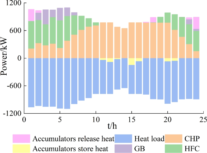
The system equipment outputs in an orderly manner within a 24-h scheduling cycle, which greatly improves energy utilization and operation economy. By solving the two-layer model, the operation plans of the system power supply, heating, gas supply and hydrogen energy system are obtained respectively, as shown in Figs. 8, 9, 10 and 11.

Figure 8 shows that wind power resources are abundant from 1:00–8:00, and the electrical load is provided by the output power of WT and HFC, supplemented by CHP. EL, as the only source of hydrogen, converts the enriched electric energy into hydrogen through high-power operation. This improves the wind power consumption rate and provides hydrogen energy supply for HFC cogeneration and MR hydrogen to methane. During periods of abundant renewable energy output, CES is charged to absorb excess renewable energy. From 9:00–19:00, when the electricity price is high and renewable energy output is insufficient, EL hydrogen production is reduced, the HFC does not work, and power output and CES output are increased through the CHP unit to meet the load demand. The CCS device absorbs the \({\text{CO}}_2\) emitted by CHP and GB in real-time throughout the scheduling cycle. This provides the MR with raw materials for hydrogen methanation. From 20:00 to 24:00, wind power gradually increases, P2G equipment consumes energy, and HFC output rises.

From Fig. 9, it is evident that the heat load demand is higher from 1:00 to 8:00, during which CHP and HFC supply the heat energy, supplemented by GB and heat storage tanks. HFC, with its zero carbon emissions, is the primary supplier of heat energy during this period. The heat load demand is lower from 9:00 to 18:00. As a result of the EL shutdown in the system, there is no hydrogen source available. Therefore, all the heat load is provided by CHP. The CHP stores the excess heat energy from the cogeneration in a heat storage tank. At 19:00–24:00, the output of renewable energy increases, and HFC starts to realize cogeneration and take over thermal energy supply.

Upon comparing Figs. 10 and 11, it is evident that the demand for hydrogen in HFC and MR comes entirely from EL electrolysis. Hydrogen is produced by EL during the hours of 1:00–10:00 and 21:00–24:00. Some of it is directly supplied to HFC for cogeneration, while the rest is produced by MR to create natural gas. The remaining hydrogen is stored in tanks and released during the high energy demand period of 19–20 h to provide HFC for cogeneration. This achieves the effect of peak shaving and valley filling, reducing the cost of energy purchase. The conversion of hydrogen to methane by MR reduces the gas purchase cost of PIES. During the period of 1:00–5:00, hydrogen energy is primarily supplied to HFC for cogeneration, and the remaining portion is used by MR and hydrogen storage tanks.

Analysis of the effect of carbon trading mechanism on PIES

In order to verify the benefits of the carbon trading model proposed in this paper, three scenarios are set up:

Scenario 4: do not consider carbon transaction cost;
Scenario 5: consider traditional ladder carbon transaction cost;
Scenario 6: consider the LCPMRP.

Table 5 Comparison of scheduling results under different scenarios.

Table 5 shows that scenario 5, which considers traditional carbon transaction costs, allows the system to obtain free carbon quotas. This results in a reduction of part of the transaction costs and a decrease of 4.54% in the system’s total PIES cost and 5.8% in system carbon emissions compared to scenario 4.

On the basis of scenario 6, a reward coefficient is introduced to give some economic compensation when the initial quota is surplus. In order to prevent excessive environmental cost, PIES operator have increased environmental cost constraints. Compared to Scenario 5, Scenario 6 reduces PIES operating costs by 1.33 % and carbon emissions by 3.29 %. Increasing the reward coefficient to reduce the carbon transaction cost can fully mobilise the enthusiasm of PIES towards carbon reduction.

Sensitivity analysis

Figure 12 shows the trend of carbon emissions and carbon transaction costs with the change of carbon price. In the range of small carbon prices, carbon price changes have little effect on unit output, and carbon emissions remain stable. However, as the cost of carbon rises, so does the cost of carbon trading. Carbon emissions are anticipated to decrease significantly as the price of carbon increases to approximately 70 yuan/t. Carbon emissions exhibit stability when the price reaches 200 yuan/t. Carbon transaction costs increase initially and subsequently decrease due to the combined impact of carbon pricing and carbon emissions. As the cost of carbon emissions increases, there is a corresponding decrease in carbon emissions.

By changing the reward and punishment coefficients, the scheduling models under different carbon prices are solved, respectively, and the results of Figure 13 are obtained. It is clear from Fig. 13 that as the carbon price increases and the incentive and punishment coefficients become larger, the cost of carbon transactions falls at a faster rate. When \(\omega \) is 0.2 and the carbon transaction price is approximately 300 yuan, the carbon transaction cost tends to remain stable. This shows that the system unit output is gradually stabilising.

Analysis of operation characteristics of CES

Figure 14 shows that CES is charged during periods of low electricity prices when power load levels are low and there are abundant wind power resources. Using CES to store excess electric energy can reduce system energy purchase costs while consuming surplus renewable energy. CES discharges during periods of high electricity prices when electric load is high, fluctuation is strong, and wind power resources are scarce. CES effectively uses the peak-valley price difference to achieve ’high incidence and low storage’ cashing. It balances the benefits of multiple stakeholders and relieves pressure on the power grid. In addition, the discharge period of CES is not only influenced by the time-of-use price of electricity, but is also related to the distribution of energy and load. It is only when the system energy supply is insufficient that CES can benefit by filling the energy shortfall.

To evaluate the impact of CES operating characteristics on the economics of each subject, the sensitivity analysis of PIES operator cost and CES operator revenue with different capacities under the deterministic model is shown in Fig. 15. The capacity of CES is adjusted to 0%, 20%, 40%,… 140% of the preset value, respectively.

Figure 15 shows that the operating cost of PIES operator shows a decreasing trend with the increase of CES capacity, because CES can effectively improve the charging enthusiasm of renewable energy surplus period. Moreover, the profit of CES shows an increasing trend, which is due to the increase of power interaction between PIES and CES. In addition, due to the limitation of CES capacity, the cost of PIES operator and the revenue of CES operator will not change after reaching a certain fixed value (minimum cost), and the CES capacity is optimal (1188 kWh). The analysis shows that an appropriate increase in CES capacity can guarantee the lowest cost for the PIES operator while increasing the revenue of the CES operator, thus achieving mutual benefits and win-win results.

Analysis of EL operating characteristics under multiple operating conditions

The production schedule of the EL array in the deterministic model is shown in Fig. 16. By analyzing the variation trend of the electric power of each EL over time, it can be seen that during the period of 1:00–6:00,22:00–24:00, when the wind power is high, most of the EL works under fluctuating production conditions, but it is allowed to work under overload production conditions for a short time, switching between overload conditions and fluctuating conditions, and absorbing the excess wind power as much as possible. This reflects that the scheduling strategy maintains the working state of the EL as much as possible on the basis of meeting energy and price fluctuations; at 8:00, in response to changes in energy prices and fluctuations in renewable energy output. The No.1 EL runs in a cold standby state for a short time, thus avoiding economic losses caused by downtime. This reflects that the model proposed in this paper takes into account the operating characteristics and start-up costs of EL, effectively reduces the number of startup and shutdown of the EL, and the operating state is more flexible.

Verification and analysis of uncertainty scheduling model based on IGDT

In this paper, other parameters are kept unchanged on the basis of the deterministic model. According to the predicted values of wind power, photovoltaic power, electric load, heat load and gas load, the entropy weights are 0.385,0.221,0.167,0.120 and 0.107 respectively. The deviation factor of the objective function is set to 0.02 steps. As the length increases from 0 to 0.20, the IGDT models based on RA and RS respectively are established.

It can be seen from Table 6 that under the RA strategy, uncertain factors have a negative impact on the PIES operator cost. As the deviation factor grows, the acceptable uncertainty of PIES gradually increases, the risk of robust optimisation decisions by operators gradually decreases, and the cost gradually increases. Under the RS strategy, uncertain factors will have a positive impact on the PIES operator cost. As the deviation factor grows, the acceptable uncertainty of PIES continues to increase, the system risk of opportunity seeking behaviour continues to increase, the system cost gradually decreases, and operators can release more operating costs. Therefore, decision makers need to set an appropriate cost deviation factor by balancing system economics and uncertainty risk.

Table 6 Sensitivity analysis of risk preference.

Figures 17 and 18 show the scheduling scheme under the RA strategy with \(\delta \) = 0.1 as an example. Figures 17 and 18 show that the IGDT robustness schedule is more conservative than the initial power schedule. The output of renewable energy is below the projected level, while the load exceeds the projected level. This can increase the pressure on the supply during periods of high system load fluctuations, resulting in insufficient supply capacity. To manage load fluctuations, the system buys electricity from the external power grid to compensate for any energy shortages. Additionally, the system increases the output of EL hydrogen production, prioritising the supply of hydrogen to HFC for cogeneration. This results in a reduction of natural gas supplied to the methane reactor and an increase in gas load. The system needs to purchase more gas energy, resulting in an increase in scheduling cost. Additionally, the reduction of renewable energy output leads to a decrease in the charging power of CES during the electricity price trough, which reduces the revenue of CES operator.

Figures 19 and 20 show the scheduling scheme under the RS strategy with \(\theta \) = 0.1 as an example. Figures 19 and 20 demonstrate that the RS method is more extreme than the output plan in the deterministic case. Because of the reduction of the electric load and the increase of the renewable energy output, the PIES operator reduces the output of the traditional unit CHP and the gas boiler. While reducing the carbon transaction cost, the consumption of natural gas is reduced, thereby reducing the gas purchase cost and the operating cost of PIES.